
Backpropagation, a fundamental concept in artificial neural networks and machine learning, operates as a supervised learning algorithm for training neural networks. The term itself stems from the process of propagating error information backward through the network. In essence, backpropagation seeks to minimize the gap between a neural network’s predicted output and the actual target values. This is achieved by adjusting the network’s weights and biases based on calculated errors. As the network iteratively refines its performance by learning from its mistakes, it becomes adept at discerning patterns and features in the data over time. 🔄 Leveraging the chain rule from calculus, backpropagation efficiently computes derivatives, guiding the iterative adjustment of weights. The process’s use of gradient descent strikes a delicate balance, enabling effective navigation through intricate weight landscapes and enhancing the network’s capacity for representation learning through implicit feature extraction in hidden layers. 🌐

In the context of neural networks, a neuron plays a crucial role in information processing. The 🧠 cell body contains the nucleus and organelles, while dendrites receive signals from other neurons. The axon transmits signals to other cells, and synapses are junctions where signals are exchanged between neurons. Weights (W1, W2, etc.) and biases (b) signify the connection strength, and the activation function determines the neuron’s output. ⚖️
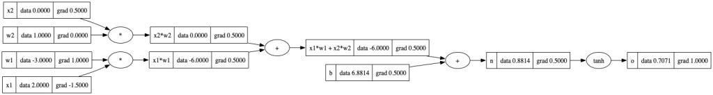
🤖 Now, let’s mimic the above NN 🧠:
# inputs x1,x2
x1 = Value(2.0, label='x1')
x2 = Value(0.0, label='x2')

# weights w1,w2
w1 = Value(-3.0, label='w1')
w2 = Value(1.0, label='w2')

# bias of the neuron
b = Value(6.8813735870195432, label='b')

# x1*w1 + x2*w2 + b
x1w1 = x1*w1; x1w1.label = 'x1*w1'
x2w2 = x2*w2; x2w2.label = 'x2*w2'

x1w1x2w2 = x1w1 + x2w2; x1w1x2w2.label = 'x1*w1 + x2*w2'
n = x1w1x2w2 + b; n.label = 'n'
o = n.tanh(); o.label = 'o'
Sure, let’s break down the above process of the forward pass in the neural network in a more detailed and easily understandable manner:
Imagine we have inputs, let’s call them x1 and x2, feeding into a two-dimensional neuron. These inputs are like messengers carrying information. Now, think of these inputs as the weights (w1, w2) assigned to the neuron. These weights act like the strength of connections, influencing how much importance we give to each input. Additionally, there’s a bias term, b, which is like a baseline for the neuron.
To compute what the neuron does, we perform a simple mathematical operation. First, we multiply each input (x1, x2) by its corresponding weight (w1, w2). This multiplication essentially scales the importance of each input. Next, we sum up these scaled inputs and add the bias term. It may seem a bit tangled, but in simpler terms, we’re just saying: ( x1 times w1 + x2 times w2 + b ).
Breaking it down even further, we take small steps to compute each part separately. We label these steps, like ( x1 times w1 ) as a variable, and ( x2 times w2 ) as another. The sum of these variables, labeled as ‘n,’ represents the raw activation, which is just a fancy way of saying the weighted sum plus bias.
Now, to make things interesting, we apply an activation function (let’s use tanh for this example) to ‘n’. This activation function is like a filter, modifying the output. So, if we call the final output ‘output,’ it’s simply the result after passing ‘n’ through the tanh activation function.
In essence, this whole process is like a neuron’s way of weighing its inputs, adding them up, and deciding whether to send a signal based on the result. The activation function adds a touch of non-linearity, introducing complexity to the neuron’s response. This seemingly complex process is the essence of a forward pass in a neural network, where the magic happens to transform inputs into meaningful outputs 🧠✨.
The reason we’re discussing the tanh activation function is because it adds a layer of complexity that our current set of operations (addition and multiplication) can’t achieve alone. Tanh is a hyperbolic function, and to implement it, we require not just addition and multiplication but also exponentiation.

Looking at the formula for tanh, you can see the involvement of exponentiation, specifically in the numerator and denominator. Without the ability to perform exponentiation, we hit a roadblock in producing the tanh function for our low-level processing node.
Now we will Add tanh to the basic operation, We can add it to the code written in the last blog post. Lets code 💻
class Value:

  def __init__(self, data, _children=(), _op='', label=''):
    self.data = data
    self.grad = 0.0
    self._prev = set(_children)
    self._op = _op
    self.label = label

  def __repr__(self):
    return f"Value(data={self.data})"

  def __add__(self, other):
    out = Value(self.data + other.data, (self, other), '+')
    return out

  def __mul__(self, other):
    out = Value(self.data * other.data, (self, other), '*')
    return out

  def tanh(self):
    x = self.data
    t = (math.exp(2*x) - 1)/(math.exp(2*x) + 1)
    out = Value(t, (self, ), 'tanh')
    return out


a = Value(2.0, label='a')
b = Value(-3.0, label='b')
c = Value(10.0, label='c')
e = a*b; e.label = 'e'
d = e + c; d.label = 'd'
f = Value(-2.0, label='f')
L = d * f; L.label = 'L'
L
Now run this code :
# inputs x1,x2
x1 = Value(2.0, label='x1')
x2 = Value(0.0, label='x2')

# weights w1,w2
w1 = Value(-3.0, label='w1')
w2 = Value(1.0, label='w2')

# bias of the neuron
b = Value(6.8813735870195432, label='b')

# x1*w1 + x2*w2 + b
x1w1 = x1*w1; x1w1.label = 'x1*w1'
x2w2 = x2*w2; x2w2.label = 'x2*w2'

x1w1x2w2 = x1w1 + x2w2; x1w1x2w2.label = 'x1*w1 + x2*w2'
n = x1w1x2w2 + b; n.label = 'n'
o = n.tanh(); o.label = 'o'
Now use the draw_dot from previous blog to visualize this graph:
draw_dot(o)
Now as long as we know the derivative of tanh, then we’ll be able to back propagate through it.
Let’s start the Backpropagation! 🚀
The derivative of ‘o’ with respect to ‘o’ is always 1.0, a fundamental rule. Now, when we draw ‘o,’ we find that the gradient is 1.0.
o.grad=1Moving to backpropagate through the tanh function, we need to know its local derivative of tanh. This derivative is:
1−tanh **2 (x)So if ‘o’ is tanh(n) , then do/dn=1- o**2 , where ‘o’ is the output of the tanh operation
i.e. .49999 ~ 0.5
n.grad=0.5Now, moving to the backpropagation process, given that dn/do is 0.5 and this is a plus node, we recall that a plus node distributes the gradient equally to both of its inputs. Therefore, the gradient for this particular step in the backpropagation is 0.5 (or 0.5 times the incoming gradient). This seamless distribution of the gradient is a characteristic of the plus node in the backpropagation process.
Since the local derivative of this operation is 1 for every node, multiplying it by 0.5 results in a gradient of 0.5 for each of the nodes in the plus operation.
x1w1x2w2.grad=0.5
b.grad=0.5
Continuing through another plus node with a distributed gradient of 0.5, we set the gradients for x2w2 and b. Since the local derivative of the plus node is 1 for every input, the 0.5 gradient is evenly distributed.
x1w1.grad=0.5
x2w2.grad=0.5
When backpropagating through a multiplication (times) node, the local derivative is the other term in the multiplication. So,
x2.grad= w2.data * x2w2.grad
w2.grad=x2.data * x2w2.grad
and similar for this :
x1.grad= w1.data * x1w1.grad
w1.grad= x1.data * x1w1.grad
The local derivative of the times operation with respect to x1 is w1, and with respect to w1 is x1. Calculating x1.grad involves multiplying w1.data by x1w1.grad, resulting in −1.5 . Similarly, w1.grad is found by multiplying x1.data by x1w1.grad, giving 1.
This provides a clear insight into the influence of each parameter on the final output. In this case, w2 doesn’t matter because its gradient is 0, but w1 is crucial. If w1 increases, the output of this neuron will go up proportionally, as indicated by the positive gradient. Understanding these gradients is fundamental to adjusting the weights during the training phase, optimizing the network’s performance.
Now visualize the final graph:
Summary ✨🔍: In this exploration of backpropagation within a neural network, we navigated through the intricate process of adjusting weights and biases to optimize model performance. Starting with the high-level understanding of backpropagation as error correction through layers, we delved into the subtleties of the process. We followed the flow of gradients, emphasizing the role of the chain rule in calculating derivatives. The blog unfolded the simplicity of backpropagation through plus and times nodes, showcasing how the local derivatives guide the adjustment of parameters. The significance of the tanh activation function and its derivative were highlighted, providing insights into its impact on the learning process. Ultimately, we witnessed the practical application of these concepts in adjusting weights to influence the output of a neuron. This journey demystified the mechanics of backpropagation, emphasizing its crucial role in the iterative learning process of neural networks.
What Next 🤔🚀:
Embark on a journey from manual to automated backpropagation in our upcoming blog. Stay tuned for a peek into the future of efficient and scalable backpropagation in our next blog installment!
Reference:
This blog is crafted with the primary goal of knowledge sharing, breaking down complex ideas into digestible concepts. It’s essential to recognize that coding, like any skill, may have its nuances. We encourage readers to view this content as a guide for learning and discovery, acknowledging the potential for minor issues during code implementation.
