You will learn to:
Build the general architecture of a learning algorithm, including:
Initializing parameters
Calculating the cost function and its gradient
Using an optimization algorithm (gradient descent)

Gather all three functions above into a main model function, in the right order.
Overview of the Problem set
Problem Statement: You are given a dataset containing:
- a training set of m_train images labeled as cat (y=1) or non-cat (y=0)
- a test set of m_test images labeled as cat or non-cat
- each image is of shape (num_px, num_px, 3) where 3 is for the 3 channels (RGB). Thus, each image is square (height = num_px) and (width = num_px).
You will build a simple image-recognition algorithm that can correctly classify pictures as cat or non-cat.
Show me the code
import numpy as np
import matplotlib.pyplot as plt
import h5py
import scipy
from PIL import Image
from scipy import ndimage
from lr_utils import load_dataset # for this lib git link is provided
%matplotlib inline
Let’s get more familiar with the dataset.In [183]:
# Loading the data (cat/non-cat)
train_set_x_orig, train_set_y, test_set_x_orig, test_set_y, classes = load_dataset()
In [28]:
train_set_x_orig.shape
Out[28]:
(209, 64, 64, 3)
In [29]:
train_set_y.shape
Out[29]:
(1, 209)
In [21]:
classes
Out[21]:
array([b'non-cat', b'cat'], dtype='|S7')
In [184]:
# Example of a picture
index = 200
plt.imshow(train_set_x_orig[index])
Out[184]:
<matplotlib.image.AxesImage at 0x22c6a3ba240>
Exercise: 1
Find the values for:
- m_train (number of training examples)
- m_test (number of test examples)
- num_px (= height = width of a training image) Remember that train_set_x_orig is a numpy-array of shape (m_train, num_px, num_px, 3). For instance, you can access m_train by writing train_set_x_orig.shape[0].
In [186]:
m_train = train_set_x_orig.shape[0]
m_test = test_set_x_orig.shape[0]
num_px = train_set_x_orig.shape[1]

print ("Number of training examples: m_train = " + str(m_train))
print ("Number of testing examples: m_test = " + str(m_test))
print ("Height/Width of each image: num_px = " + str(num_px))
print ("Each image is of size: (" + str(num_px) + ", " + str(num_px) + ", 3)")
print ("train_set_x shape: " + str(train_set_x_orig.shape))
print ("train_set_y shape: " + str(train_set_y.shape))
print ("test_set_x shape: " + str(test_set_x_orig.shape))
print ("test_set_y shape: " + str(test_set_y.shape))
Number of training examples: m_train = 209
Number of testing examples: m_test = 50
Height/Width of each image: num_px = 64
Each image is of size: (64, 64, 3)
train_set_x shape: (209, 64, 64, 3)
train_set_y shape: (1, 209)
test_set_x shape: (50, 64, 64, 3)
test_set_y shape: (1, 50)
Exercise:2
Standardize and Reshape the training and test data sets so that images of size (num_px, num_px, 3) are flattened into single vectors of shape (num_px ∗ num_px ∗ 3, 1).In [66]:
train_set_x_flatten =train_set_x_orig.reshape(train_set_x_orig.shape[1]*train_set_x_orig.shape[1]*3,train_set_x_orig.shape[0])
In [67]:
train_set_x_flatten .shape
Out[67]:
(12288, 209)
In [54]:
test_set_x_flatten =test_set_x_orig.reshape(test_set_x_orig.shape[1]*test_set_x_orig.shape[1]*3,test_set_x_orig.shape[0])
In [56]:
test_set_x_flatten.shape
Out[56]:
(12288, 50)
To represent color images, the red, green and blue channels (RGB) must be specified for each pixel, and so the pixel value is actually a vector of three numbers ranging from 0 to 255. Let’s standardize our dataset.In [69]:
train_set_x = train_set_x_flatten/255.
test_set_x = test_set_x_flatten/255.
General Architecture of the learning algorithm
- Initialize the parameters of the model
- Learn the parameters for the model by minimizing the cost
- Use the learned parameters to make predictions (on the test set)
- Analyse the results and conclude
Building the parts of our algorithm
The main steps for building a Neural Network are: Define the model structure (such as number of input features) Initialize the model’s parameters Loop: Calculate current loss (forward propagation) Calculate current gradient (backward propagation) Update parameters (gradient descent) You often build 1-3 separately and integrate them into one function we call model().
Exercise:3
Implement sigmoid() function .In [188]:
def sigmoid(z):
    return 1/(1+np.exp(-z))
In [189]:
print ("sigmoid([0, 2]) = " + str(sigmoid(np.array([0,2]))))
sigmoid([0, 2]) = [0.5 0.88079708]
Initializing parameters
Exercise:4
Implement parameter initialization. You have to initialize w as a vector of zeros. If you don’t know what numpy function to use, look up np.zeros() in the Numpy library’s documentation.In [192]:
def initialize_with_zeros(dim):
    w=np.zeros((dim,1))
    b=0
    return w,b
In [193]:
dim = 5
w, b = initialize_with_zeros(dim)
print ("w = " + str(w))
print ("b = " + str(b))
w = [[0.]
 [0.]
 [0.]
 [0.]
 [0.]]
b = 0
Forward and Backward propagation
Exercise:5
Implement a function propagate() that computes the cost function and its gradient.In [194]:
def propagate(w, b, X, Y):
    m=X.shape[1]
    A=sigmoid((np.dot(w.T,X) + b))
    yloga=np.multiply(Y,np.log(A))
    ylogaa=np.multiply((1-Y),np.log(1-A))
    cost=(-1/m)*(np.sum(yloga+ylogaa))
    dw=(1/m)*(np.dot(X,(A-Y).T))
    db=(1/m)*(np.sum(A-Y))
    assert(dw.shape == w.shape)
    assert(db.dtype == float)
    cost = np.squeeze(cost)
    assert(cost.shape == ())
    grads = {"dw": dw,
             "db": db}
    return grads, cost
In [195]:
w, b, X, Y = np.array([[1.],[2.]]), 2., np.array([[1.,2.,-1.],[3.,4.,-3.2]]), np.array([[1,0,1]])
grads, cost = propagate(w, b, X, Y)
print ("dw = " + str(grads["dw"]))
print ("db = " + str(grads["db"]))
print ("cost = " + str(cost))
dw = [[0.99845601]
 [2.39507239]]
db = 0.001455578136784208
cost = 5.801545319394553
Optimization
You have initialized your parameters. You are also able to compute a cost function and its gradient. Now, you want to update the parameters using gradient descent.
Exercise: 6
Write down the optimization function. The goal is to learn w and b by minimizing the cost function J . For a parameter θ ,the update rule is θ=θ−α*dθ ,where α is the learning rate.In [196]:
def optimize(w, b, X, Y, num_iterations, learning_rate, print_cost = False):
    costs=[]
    for i in range(num_iterations):
        grads, cost=propagate(w, b, X, Y)

        dw=grads['dw']
        db=grads['db']

        w=w-np.multiply(learning_rate,dw)
        b=b-np.multiply(learning_rate,db)

        costs.append(cost)

        # Record the costs
        if i % 100 == 0:
            costs.append(cost)

        # Print the cost every 100 training iterations
        if print_cost and i % 100 == 0:
            print ("Cost after iteration %i: %f" %(i, cost))

    params = {"w": w,
              "b": b}
    grads = {"dw": dw,
             "db": db}
    return params, grads, costs
In [197]:
params, grads, costs = optimize(w, b, X, Y, num_iterations= 100, learning_rate = 0.009, print_cost = False)

print ("w = " + str(params["w"]))
print ("b = " + str(params["b"]))
print ("dw = " + str(grads["dw"]))
print ("db = " + str(grads["db"]))
w = [[0.19033591]
 [0.12259159]]
b = 1.9253598300845747
dw = [[0.67752042]
 [1.41625495]]
db = 0.21919450454067652
Exercise: 7
We are able to learned w and b for a dataset X. Now Implement the predict() function.In [147]:
def predict(w, b, X):
    m = X.shape[1]
    Y_prediction = np.zeros((1,m))
    A=sigmoid(np.dot(w.T,X)+b)
    for i in range(A.shape[1]):
            if A[0,i] > 0.5:
                Y_prediction[0][i] = 1
            else:
                Y_prediction[0][i] = 0
    assert(Y_prediction.shape == (1, m))
    return Y_prediction
In [148]:
w = np.array([[0.1124579],[0.23106775]])
b = -0.3
X = np.array([[1.,-1.1,-3.2],[1.2,2.,0.1]])
print ("predictions = " + str(predict(w, b, X)))
predictions = [[1. 1. 0.]]
Merge all functions into a model
You will now see how the overall model is structured by putting together all the building blocks (functions implemented in the previous parts) together, in the right order.
Exercise: Implement the model function. Use the following notation:
- Y_prediction_test for your predictions on the test set
- Y_prediction_train for your predictions on the train set
- w, costs, grads for the outputs of optimize()
In [198]:
def model(X_train, Y_train, X_test, Y_test, num_iterations = 2000, learning_rate = 0.5, print_cost = False):
    dim=X_train.shape[0]
    w,b=initialize_with_zeros(dim)
    params, grads, costs = optimize(w, b, X_train, Y_train, num_iterations= num_iterations, learning_rate= learning_rate, print_cost= True)

    Y_prediction_train=predict(params["w"], params["b"], X_train)
    Y_prediction_test=predict(params["w"],params["b"], X_test)

    print("train accuracy: {} %".format(100 - np.mean(np.abs(Y_prediction_train - Y_train)) * 100))
    print("test accuracy: {} %".format(100 - np.mean(np.abs(Y_prediction_test - Y_test)) * 100))

    d = {"costs": costs,
         "Y_prediction_test": Y_prediction_test,
         "Y_prediction_train" : Y_prediction_train,
         "w" : params["w"],
         "b" : params["b"],
         "learning_rate" : learning_rate,
         "num_iterations": num_iterations}

    return d
In [203]:
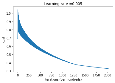
d=model(train_set_x, train_set_y, test_set_x, test_set_y, num_iterations = 2000, learning_rate = 0.005, print_cost = True)
Cost after iteration 0: 0.693147
Cost after iteration 100: 0.709726
Cost after iteration 200: 0.657712
Cost after iteration 300: 0.614611
Cost after iteration 400: 0.578001
Cost after iteration 500: 0.546372
Cost after iteration 6: 0.518331
Cost after iteration 700: 0.492852
Cost after iteration 800: 0.469259
Cost after iteration 900: 0.447139
Cost after iteration 1000: 0.426262
Cost after iteration 1100: 0.406617
Cost after iteration 1200: 0.388723
Cost after iteration 1300: 0.374678
Cost after iteration 1400: 0.365826
Cost after iteration 1500: 0.358532
Cost after iteration 1600: 0.351612
Cost after iteration 1700: 0.345012
Cost after iteration 1800: 0.338704
Cost after iteration 1900: 0.332664
train accuracy: 91.38755980861244 %
test accuracy: 34.0 %
In [162]:
# Plot learning curve (with costs)
costs = np.squeeze(d['costs'])
plt.plot(costs)
plt.ylabel('cost')
plt.xlabel('iterations (per hundreds)')
plt.title("Learning rate =" + str(d["learning_rate"]))
plt.show()
In [165]:
classes
Out[165]:
array([b'non-cat', b'cat'], dtype='|S7')
In [175]:
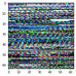
# Example of a picture that was wrongly classified.
index = 2
plt.imshow(test_set_x[:,index].reshape((num_px, num_px, 3)))
# print ("y = " + str(test_set_y[0,index]) + ", you predicted that it is a \"" + classes[d["Y_prediction_test"][0,index]].decode("utf-8") +  "\" picture.")
Out[175]:
<matplotlib.image.AxesImage at 0x22c6a2d2f60>
In [ ]:
learning_rates = [0.01, 0.001, 0.0001]
models = {}
for i in learning_rates:
    print ("learning rate is: " + str(i))
    models[str(i)] = model(train_set_x, train_set_y, test_set_x, test_set_y, num_iterations = 1500, learning_rate = i, print_cost = False)
    print ('\n' + "-------------------------------------------------------" + '\n')

for i in learning_rates:
    plt.plot(np.squeeze(models[str(i)]["costs"]), label= str(models[str(i)]["learning_rate"]))

plt.ylabel('cost')
plt.xlabel('iterations (hundreds)')

legend = plt.legend(loc='upper center', shadow=True)
frame = legend.get_frame()
frame.set_facecolor('0.90')
plt.show()
learning rate is: 0.01
Cost after iteration 0: 0.693147
Cost after iteration 100: 2.321788
Cost after iteration 200: 3.011239
Cost after iteration 300: 0.483519
Cost after iteration 400: 1.297533
Cost after iteration 500: 1.215430
Cost after iteration 600: 1.135770
Cost after iteration 700: 0.901737
Cost after iteration 800: 0.821976
Cost after iteration 900: 0.791033
Cost after iteration 1000: 0.762400
Cost after iteration 1100: 0.736228
Cost after iteration 1200: 0.711983
Cost after iteration 1300: 0.689076
Cost after iteration 1400: 0.667013
train accuracy: 71.29186602870814 %
test accuracy: 64.0 %

-------------------------------------------------------

learning rate is: 0.001
Cost after iteration 0: 0.693147
Cost after iteration 100: 0.605784
Cost after iteration 200: 0.589938
Cost after iteration 300: 0.577890
Cost after iteration 400: 0.567791
Cost after iteration 500: 0.559013
Cost after iteration 600: 0.551207
Cost after iteration 700: 0.544146
Cost after iteration 800: 0.537671
Cost after iteration 900: 0.531668
Cost after iteration 1000: 0.526054
Cost after iteration 1100: 0.520764
Cost after iteration 1200: 0.515752
Cost after iteration 1300: 0.510979
Cost after iteration 1400: 0.506416
train accuracy: 74.16267942583733 %
test accuracy: 34.0 %

-------------------------------------------------------

learning rate is: 0.0001
Cost after iteration 0: 0.693147
Cost after iteration 100: 0.636292
Cost after iteration 200: 0.630322
Cost after iteration 300: 0.625487
Cost after iteration 400: 0.621470
Cost after iteration 500: 0.618051
Cost after iteration 600: 0.615075
Cost after iteration 700: 0.612432
Cost after iteration 800: 0.610042
Cost after iteration 900: 0.607850
Cost after iteration 1000: 0.605814
Cost after iteration 1100: 0.603904
Cost after iteration 1200: 0.602098
Cost after iteration 1300: 0.600377
Cost after iteration 1400: 0.598731
lr_utils.py code
import numpy as np
import h5py

def load_dataset():
 train_dataset = h5py.File('datasets/train_catvnoncat.h5', "r")
 train_set_x_orig = np.array(train_dataset["train_set_x"][:]) # your train set features
 train_set_y_orig = np.array(train_dataset["train_set_y"][:]) # your train set labels
 test_dataset = h5py.File('datasets/test_catvnoncat.h5', "r")
 test_set_x_orig = np.array(test_dataset["test_set_x"][:]) # your test set features
 test_set_y_orig = np.array(test_dataset["test_set_y"][:]) # your test set labels

 classes = np.array(test_dataset["list_classes"][:]) # the list of classes

 train_set_y_orig = train_set_y_orig.reshape((1, train_set_y_orig.shape[0]))
 test_set_y_orig = test_set_y_orig.reshape((1, test_set_y_orig.shape[0]))

 return train_set_x_orig, train_set_y_orig, test_set_x_orig, test_set_y_orig, classes
REFERENCES:
coursera.org
deep learning specialization
